Overcoming Deep Double Descent Using PerceptiLabs

If you've ever heard the phrase: "this is gonna get worse before it gets better", then you're already halfway there to understanding Deep Double Descent.

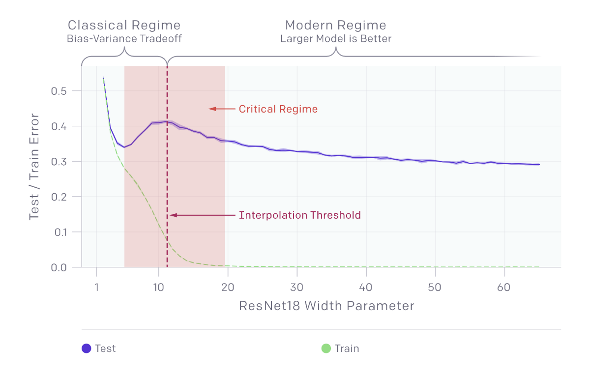
In 2019, Open AI published a great article about the Deep Double Descent phenomenon. It nicely sums up how the loss (error) for models like CNNs and ResNets, tends to improve, get worse, and then improve again, while you iterate on your model during training and testing.

Ironically, even the most knowledgeable DL researchers are struggling to understand the underlying reasons why this fascinating phenomenon occurs.

Three Deep Double Descent Scenarios

Open AI's article calls out three scenarios where Deep Double Descent generally shows itself, namely:

• Model-wise Double Descent: the model is initially under-parameterized (i.e., it needs additional complexity and hyperparameters), but continually improves after a sufficient number of parameter updates are made, such as changes to the optimizer, number of training samples, or label noise.

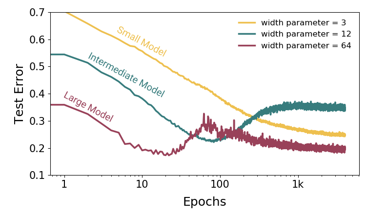
• Epoch-wise Double Descent: under-parameterized models experience a monotonic decrease in error as training time (i.e., number of epochs) is increased, while larger models must be trained across a sufficiently large, but not too large, number of epochs to find the optimal error.

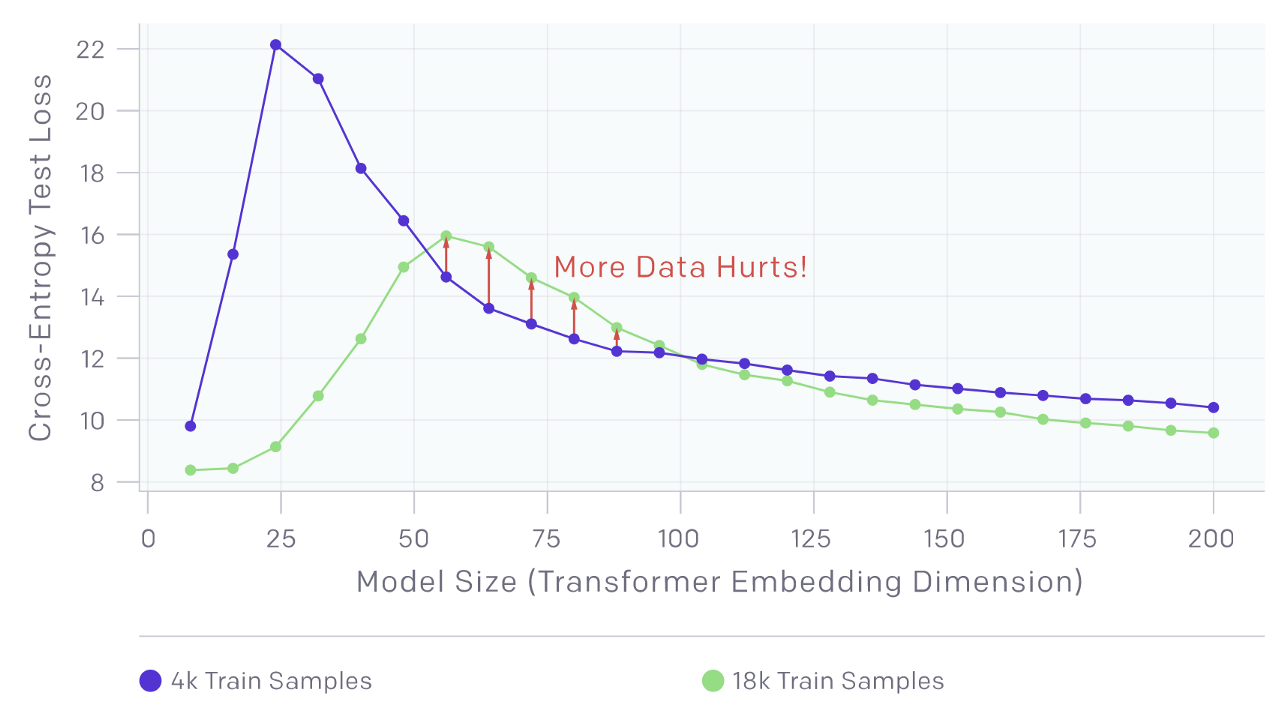
• Sample-wise Non-monotonicity: the model's performance initially decreases as the amount of data is increased, such that the transition from lower to higher model performance requires more data.

Overcoming the Odds

Understanding these three scenarios is important, but equally important, is knowing how to identify and overcome them, given your chosen ML toolset and framework.

As the old saying goes: "the first step is admitting that you've got a problem". In this case, that "problem" lies in identifying and chasing down trends in model error changes that even experienced researchers struggle to provide explanations for.

Overcoming them involves selecting the right dataset and size, model architecture, and training procedure while iterating. Thankfully, this is a case where PerceptiLabs users have it good, because our low-code environment makes adjusting all of these aspects easy while experimenting with your model. Let's look at a few approaches and features of PerceptiLabs that can support you when dealing with Deep Double Descent.

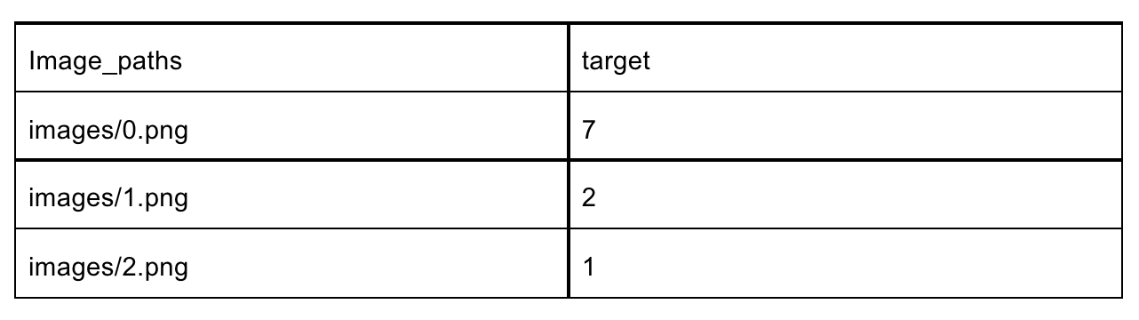
The first step in this process is to closely watch your dataset size. PerceptiLabs' Data Wizard makes it easy to set the number of samples by specifying them in your dataset's CSV file. These CSV files allow you to map your unstructured data (e.g., images) to classifications. Figure 4 below shows a very small example of a CSV used to load image data and the corresponding classification labels into PerceptiLabs:

This can be configured when you first import your data, and at any time afterwards from within the Modeling Tool, as shown in Figure 5:

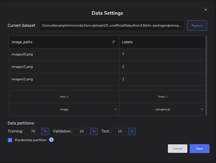
Within this popup, you can modify or reload your CSV to change the data samples and/or quantities loaded into your model, as well as change how that data is distributed for training, validation, and testing.

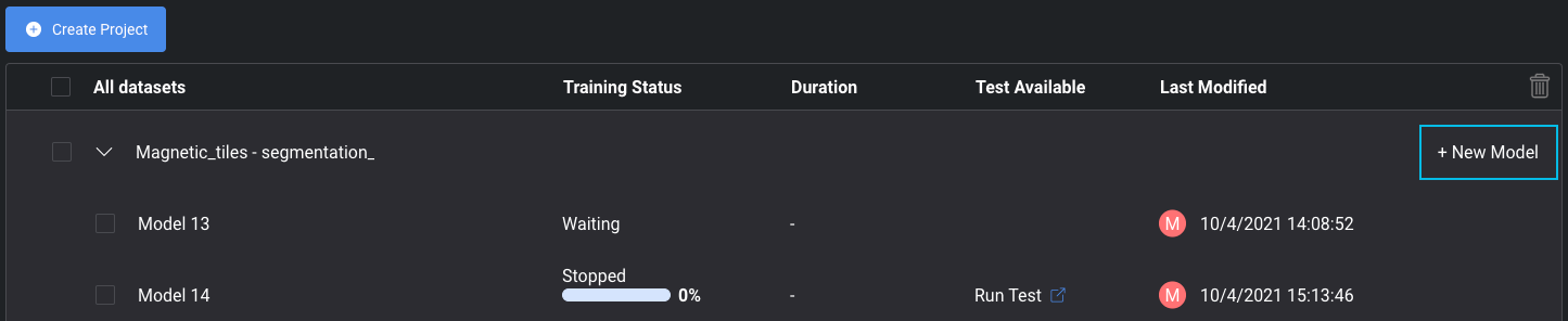
You can also easily create new models for the same dataset using the Model Hub, which makes it easy to experiment and compare different settings across models as shown here:

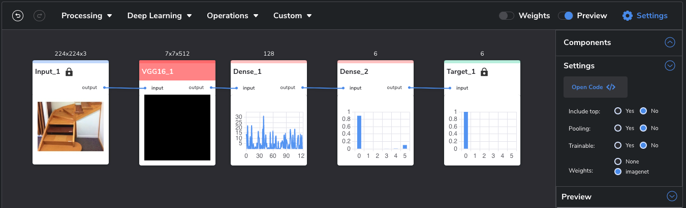
The next step of course, is the model architecture itself, which defines the complexity of the model and ultimately, the number of hyperparameters. PerceptiLabs generates a default model for you with good baseline settings when you initially import your data. You can then easily change the architecture by adding/replacing Components and/or adjusting Component settings like the activation function and dropout. And if you're using a Component like VGG16, that allows for easy transfer learning, you can choose whether to employ pre-trained weights such as those from ImageNet:

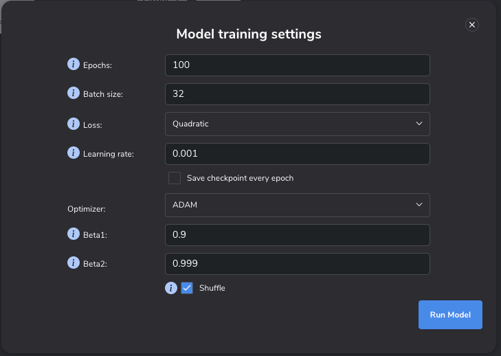
Finally, it's time to adjust the model's training settings. These settings are accessible when you run your model, so you can experiment with adjusting the number of epochs, loss function, and the optimizer – see Figure 8:

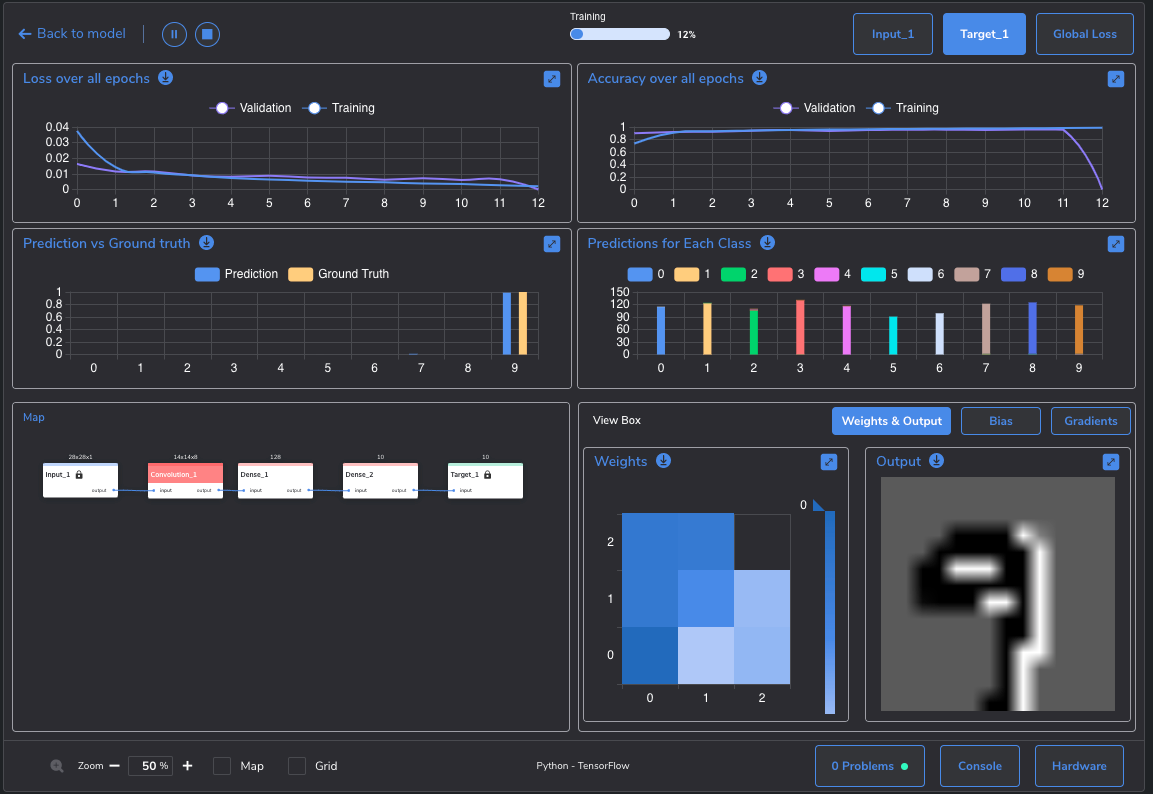
With this plethora of adjustments, the fun – or hard work, depending on your viewpoint – begins. During your training, you'll need to keep a close eye on the loss, and record it across training sessions for comparison. For that you'll use the Loss pane in PerceptiLabs' rich Statistic View that is displayed during training. The Loss pane can be displayed by selecting the Target box near the upper right of the Statistics View:

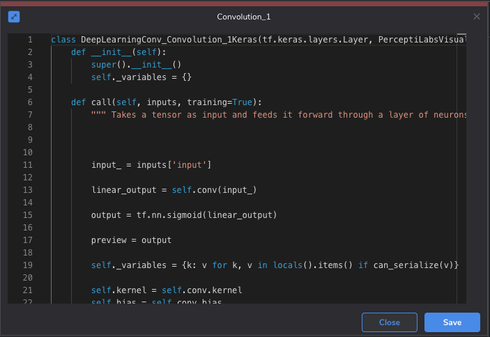
In case you haven't noticed so far, all of the aforementioned adjustments can be done without writing or modifying any code. If you're more of a low-code person, PerceptiLabs gives you full access to the underlying TensorFlow code that you can edit. By accessing the Code Editor for each Component, you can adjust most of the settings (other than data and training settings), and even a Component's logic, on the fly:

Conclusion

Deep Double Descent can occur for many reasons but even knowledgeable DL researchers still struggle to explain the phenomenon’s underpinnings. So, knowing that it can occur in your project, and the different factors which affect it, is important. Thankfully PerceptiLabs' low-code visual approach to DL modeling provides a rich set of tools for dealing with this phenomenon.

For additional information, check out The Double Descent Hypothesis: How Bigger Models and More Data Can Hurt Performance on KDnuggets, which provides additional insight into that OpenAI article we mentioned earlier. And for a deeper dive, check out the paper: Deep Double Descent: Where Bigger Models and More Data Hurt by Nakkiran et Al.

And be sure to check out our Quickstart Guide today to get started with PerceptiLabs. You'll be up and running in no time!