Use Case: A Voice Recognition model using Image Recognition

Say what? Yes you heard right – we created a model for voice recognition using image recognition.

Spoken language is the most natural form of human interaction, and thanks to advancements in modern-day ML, it's fast becoming the perfect way to interact with computers. This voice recognition is very useful for hands-free interactions and has demonstrated high accuracy and performance in small devices such as with Google and Alexa voice assistants.

One of the key challenges for a voice recognition system is to discern commands from speech samples captured in noisy environments. While traditional digital signal processing (DSP) approaches employ classic statistical methods (e.g., to filter out noise), ML takes a different approach by training models using noisy samples to classify the word(s) represented in a given speech clip.

Since audio data can be visually represented using spectrograms, we thought this would be a perfect use case to test with Perceptilabs. To demonstrate this, we built and trained an image recognition model on spectrograms representing the words "yes" and "no", which were generated from audio files containing these spoken words and some degree of noise. Let's ‘see’ how we did with our model.

Dataset

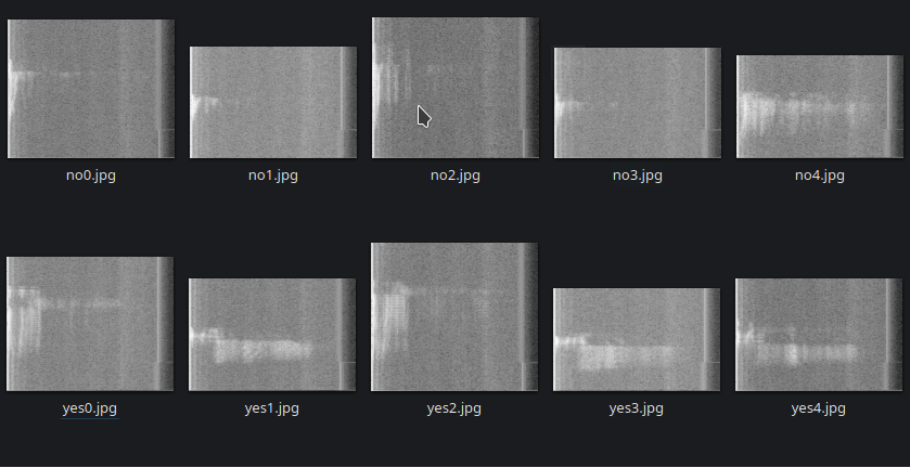
We started by looking for a set of audio files containing "yes" and "no" speech samples and eventually found just what we were looking for in this GitHub repo. Its dataset comprises 1600 16-bit stereo .wav files which we reduced down to 800 (400 for "yes" and 400 for "no") and converted to mono. We then created a Jupyter Notebook file to generate spectrograms in grayscale .jpg format for each audio file. Figure 1 shows a few example spectrograms that we generated:

To map the classifications (yes and no) to the images, we created a .csv file that associates each image file with the appropriate classification label for use in loading the data via PerceptiLabs' Data Wizard. Below is a partial example of how the .csv file looks:

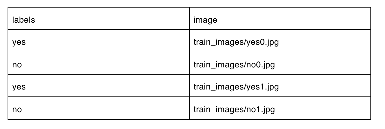
We've made the image data and this CSV file available for experimentation on GitHub.

Model Summary

Our model was built with the following Components:

Figure 2 shows the model's topology in PerceptiLabs:

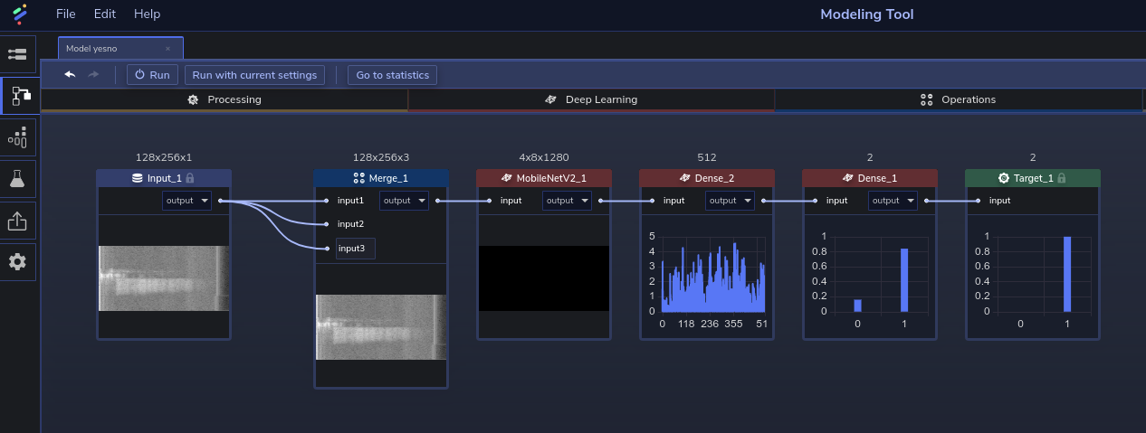
We chose to use a MobileNetV2 pre-trained with ImageNet due to its inference performance on mobile and small devices. In the model you can see that we inserted a Merge Component between the Input and MobileNetV2 components. This was used for transforming the grayscale image into an RGB image so it can be used in the pre-trained MobileNetV2 component, since the pre-trained MobileNetV2 component requires RGB inputs.

Note: since the input images are of varying sizes, we configured the pre-processing pipeline in PerceptiLabs' Data Wizard to transform the images so that they're all the same size.

Training and Results

We trained the model with 10 epochs in batches of 32, using the ADAM optimizer, a learning rate of 0.001, and a Cross Entropy loss function. With a training time of around 131 seconds, we were able to achieve a training and validation accuracy of 100%. Figure 3 shows the results after training:

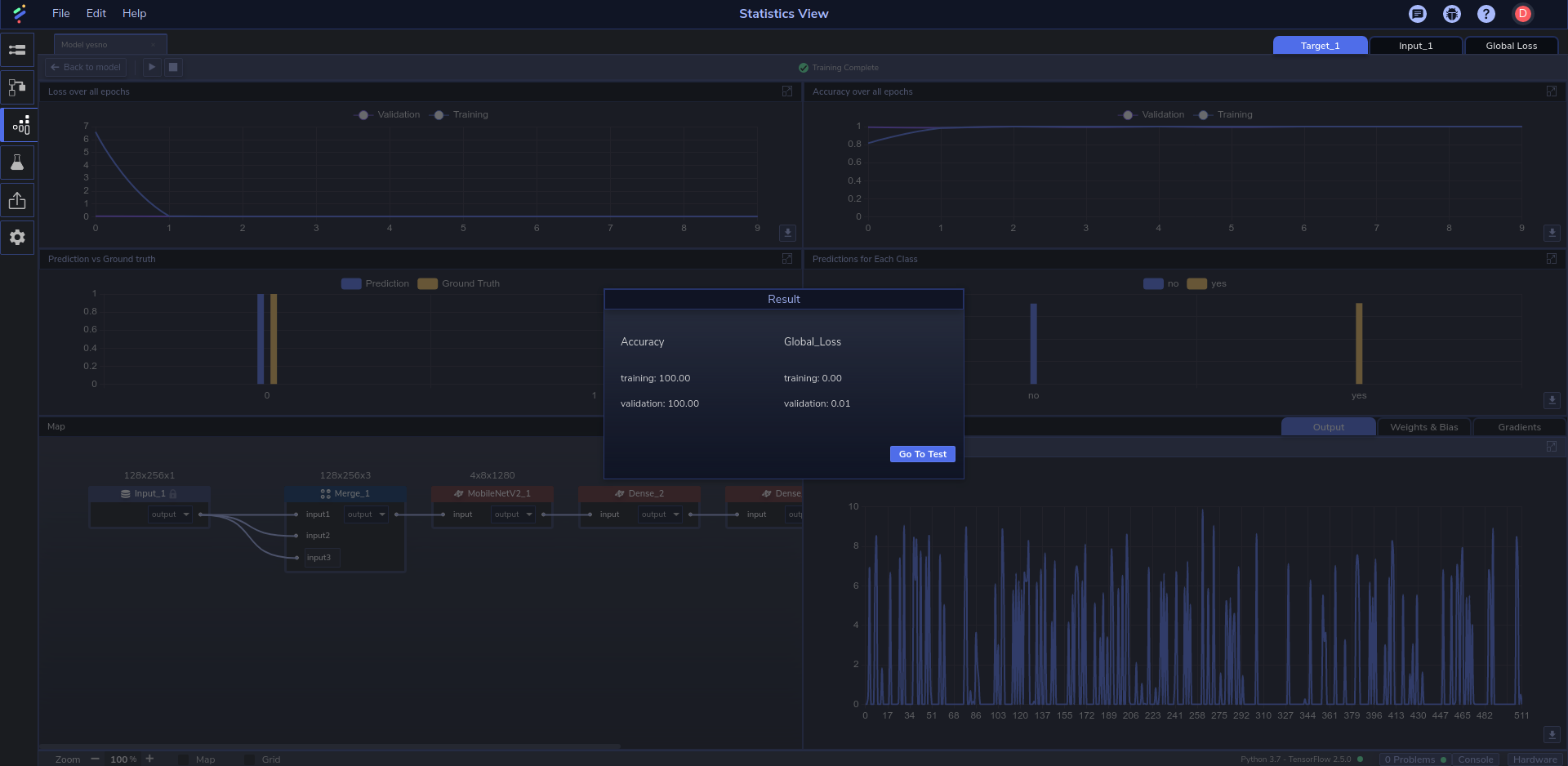
Figure 4 below shows the accuracy and loss for both validation and training:

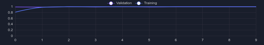
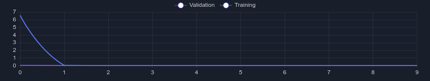
Here, we can see that accuracy ramped up quickly for training over the first epoch before stabilizing at 1, while validation accuracy started and remained at 1. Training loss quickly dropped to 0 over the first epoch while validation loss started and remained at 0.

Figure 5 below shows the Confusion Matrix and Label Metrics Table test results for the model:

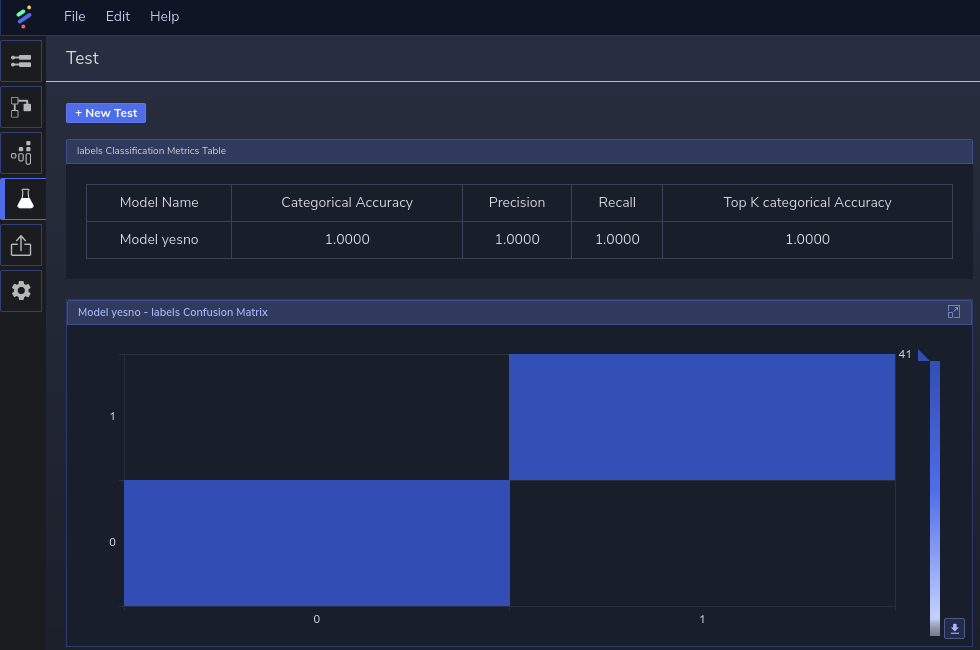
The Confusion Matrix indicates that the model tests all samples correctly (i.e., there are no false positives or negatives). The Labels Metrics Table further corroborates this by showing normalized values of 1.0 (i.e., 100%) for the following: Categorical accuracy (accuracy for each category averaged over all of them), Top K Categorical Accuracy (frequency of the correct category among the top K predicted categories), Precision (accuracy of positive predictions), and Recall (percentage of positives found (i.e., not misclassified as negatives instead of positives).

Vertical Applications

A model like this could be used as the basis for voice recognition applications and voice user interfaces. If trained with additional speech samples, the model could be used to build new types of personal assistants and hands-free applications. Examples in different verticals include:

• Automotive: in-car infotainment systems that incorporate voice commands to make calls, change the in-car temperature, etc.
• AR: applications for technicians who use AR to provide additional information about a mechanical system that they're repairing using their hands. Here, a hands-free VUI allows the technician to navigate menus in the display through spoken commands while continuing to service the mechanical system.
• Wearables: smart wrist watch applications can detect spoken commands to perform different functions.

The model could also be used as the basis for transfer learning to create new models that can make predictions from images of other types of signal data (e.g., other types of sounds, heatmaps, light data, etc.).

Summary

This use case is an example of how PerceptiLabs' strengths in building image recognition models can be used for voice recognition applications. For inference, you would likely employ some sort of real-time audio-to-spectrogram system that can generate image data to run inference on, rather than rely on a Jupyter Notebook to perform the conversion. However, the Jupyter Notebook we created provides a convenient foundation for building training samples.

One of the benefits of using ML instead of classic statistics-based DSP for voice recognition, is that you can use Convolutional layers which are highly efficient, scalable, and have some nice properties depending on their setup. For example, they offer translation invariance, which means it doesn't matter if an object (e.g., voice data) appears on the left or right part of the image, it's still treated the same.
If you want to build a deep learning model similar to this, run PerceptiLabs and grab a copy of our pre-processed dataset from GitHub.