Use Case: Wildfire Detection

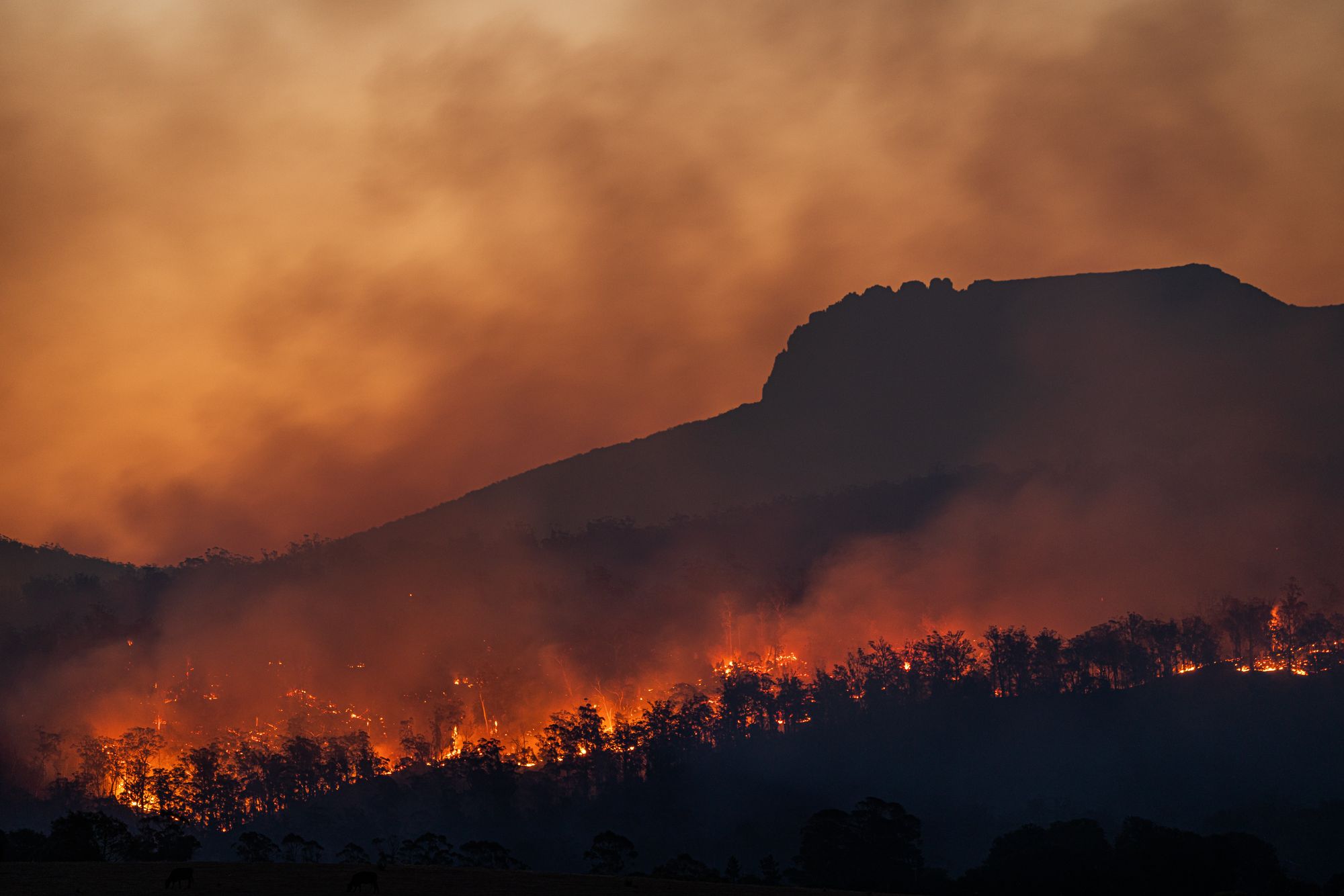
Every year, millions of hectares of forest are lost due to the spread of wildfires. However, using image recognition, authorities may now be able to identify wildfires from live-streamed images from cameras on highways or buildings.

Inspired by the potential to help save the environment using deep learning, we built an image recognition model in PerceptiLabs that could analyze images of scenes to detect fires. Governments or environmental groups could potentially use such a model to alert firefighters before a fire spreads too far.

Dataset

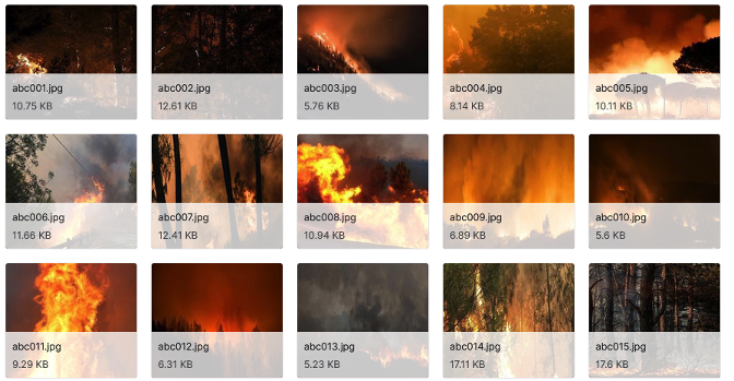
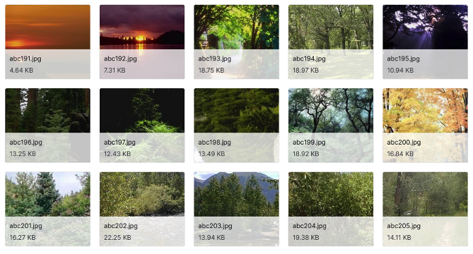
To train our model, we used images from Wildfire Detection Image Data on Kaggle¹. This dataset comprises 1900, 250x250 pixel .jpg files, some of which are shown in Figure 1:

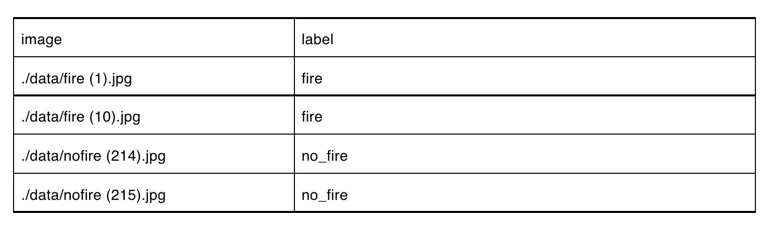
To classify these images, we devised two classification labels: fire and no_fire, and created a .csv file to associate them with each image file for loading the data using PerceptiLabs' Data Wizard. Below is a partial example of how the .csv file looks:

Model Summary

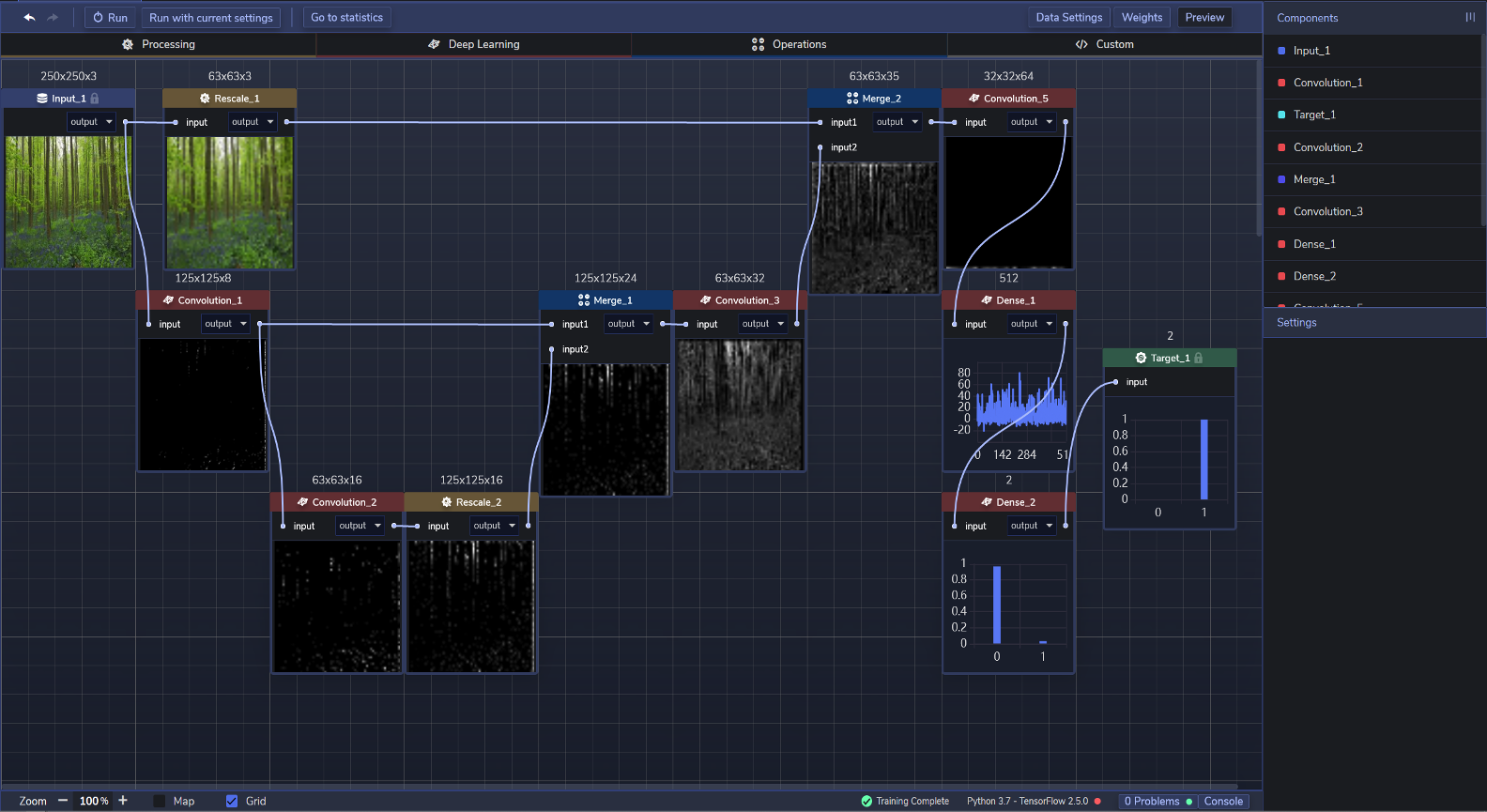
For our model, we built a CNN model comprising the following Components:

The model, shown in Figure 2 below, is essentially a small U-Net variant, with similar benefits from the skip connections that a standard U-Net would have. With this architecture, we convolve and pool the image in the contraction path into feature maps while using the skip connections to pass information to the expansive path. The expansive path then combines feature information together with spatial information before using fully-connected layers (Dense Components) for binary classification into fire and no_fire.

Figure 2 shows the model's topology in PerceptiLabs:

Training and Results

We trained the model in batches of 32 across three epochs, using the ADAM optimizer, a learning rate of 0.001, and a Cross-Entropy loss function. With an average training time of around 269.73 seconds, we achieved a training accuracy of 97.82% and a validation accuracy of 96.05%:

Figure 3 shows PerceptiLabs' Statistics view:

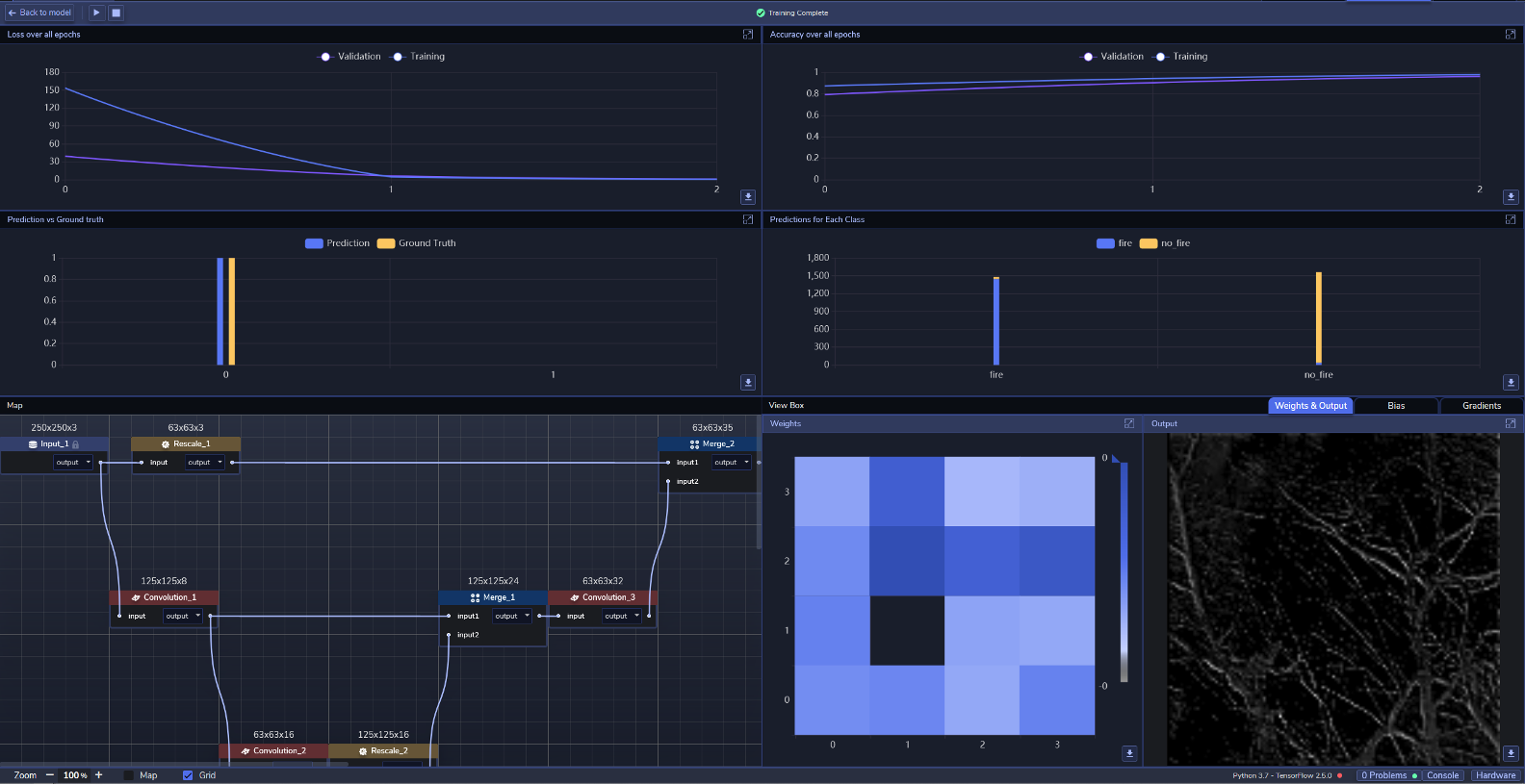
Figures 4 and 5 below show the accuracy and loss across the epochs:

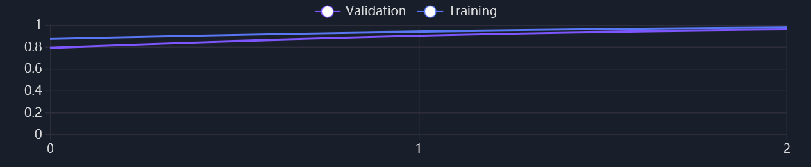
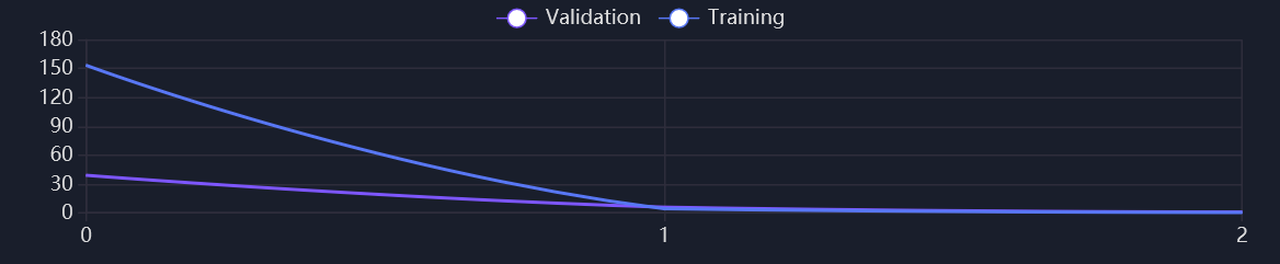
In Figure 4, we can see that the accuracy for both training and validation started relatively high and increased at about the same rates. In Figure 5, training loss started high, and validation loss started much lower, but both ended up being about the same by the second epoch.

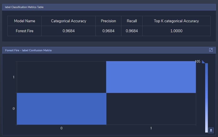
The Confusion Matrix in Figure 6 shows two very similar shades of blue, indicating that the model tests all samples correctly almost all of the time. The Labels Metrics Table corroborates this by showing normalized values just shy of 97% for the following: Categorical accuracy (accuracy for each category averaged over all of them), Precision (accuracy of positive predictions), and Recall (percentage of positives found (i.e., not misclassified as negatives instead of positives) and 100% for Top K Categorical Accuracy (frequency of the correct category among the top K predicted categories).

Vertical Applications

A model like this could be used as the basis for analyzing different types of environmental imagery to detect anomalies. By using this model for transfer learning, you could potentially develop models for detecting other types of issues such as flooding, erosion, or mudslides. It could also be modified to work on other data types like satellite imagery to detect unauthorized deforestation, rising water levels, or melting icebergs.

Try it for yourself!

We've made everything that you need to try this out yourself available on GitHub.

Using PerceptiLabs, you can quickly load this data via the Data Wizard and construct a model like this using the settings above, all without writing any code. Or, use the model.json file that we've included to directly import our model into PerceptiLabs (requires PerceptiLabs 0.12.0 or higher). Either way, you'll be up and running in no time!

You can then easily swap over to a different dataset for training on that new data, and/or adjust your model's topology with new Components and connections. Your trained model can then be exported with just a few clicks, after which, the model files can be hosted by your application for real-world inference.

Summary

This use case is an example of how image recognition can be used for detecting dangerous environmental conditions. If you want to build a deep learning model similar to this, run PerceptiLabs and check out the repo we created for this use case on GitHub. And for another environmental use case, be sure to check out Automated Weather Analysis Using Image Recognition.

¹Dataset Credits: Baris Dincer (2021), Wildfire Detection Image Data For Machine Learning Process, Kaggle, V1, https://www.kaggle.com/brsdincer/wildfire-detection-image-data, Database Contents License (DbCL) v1.0